 Abstract
We propose PhysMorph‑GS, an end‑to‑end framework that optimizes internal physics controls directly from image‑space losses.
•
Beyond initial-state tuning. Instead of only optimizing how a simulation starts, we optimize how it evolves over time by learning a sequence of control deformation gradients F~p\tilde{F}_pF~p.
•
Appearance‑driven physics control. A high‑level visual target (silhouette + depth of a desired shape) is converted into low‑level physical controls, aligning the MPM deformation field with the rendered images while preserving mass and material behavior.
•
Bidirectional physics–rendering bridge. Differentiable MPM and 3D Gaussian Splatting (3DGS) are coupled through a deformation‑aware upsampling bridge so that pixel‑space gradients flow back to both particle positions and deformation gradients.
Technical Pipeline
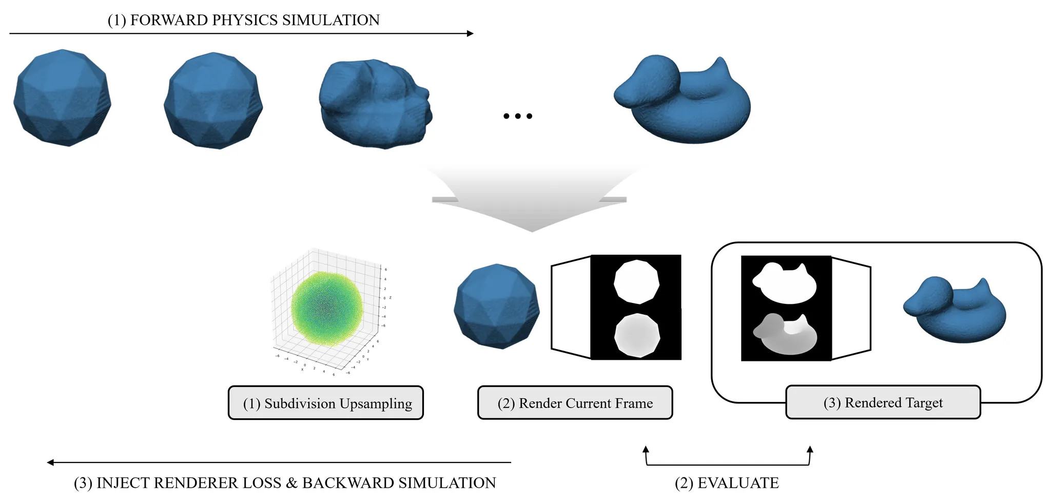
High‑level summary
We build a fully differentiable loop:MPM (C++) → sparse physics state (x_low, F_low) → deformation‑aware upsampling & F‑smoothing → Gaussian covariance construction (μ, Σ) → 3DGS rendering + image losses → gradients back to controls F
More concretely:
1.
Forward physics pass (C++ / DiffMPM)
•
A differentiable MLS‑MPM solver runs a forward simulation under the current control sequence (dFc).
•
For each timestep we obtain anchor particle positions xlowx_{\text{low}}xlow and deformation gradients FlowF_{\text{low}}Flow.
2.
State transfer (C++ → Python)
•
Via pybind11, the anchor states are exposed to Python as NumPy arrays.
•
These anchors carry all physical mass and momentum; everything created later is render‑only.
3.
Surface‑aware upsampling (sparse physics → dense surface samples)
From the sparse volumetric MPM state we synthesize a dense set of render particles:
•
Soft surface gating. PCA‑based sheetness + percentile statistics + EMA + hysteresis produce a soft probability psurfp_{\text{surf}}psurf of being on or near the surface.
•
Density map & sampling. We build a spatial density map from and deformation magnitude , then sample new particles using a differentiable top‑K Gumbel‑Softmax style selection so that high‑strain, high‑visibility regions receive more samples.
4.
Multi‑scale deformation field & covariance construction
•
We interpolate a multi‑scale F‑field from anchors to render particles (coarse/fine k‑NN + edge‑aware blending), obtaining smoothed deformation gradients FrenderF_{\text{render}}Frender on the dense set.
•
For each render particle we build an anisotropic Gaussian:
◦
,
so the covariance encodes physical stretch/compression but not rotation.
5.
Differentiable 3DGS rendering
•
The Gaussians are rendered with a 3DGS rasterizer under a known camera and lighting setup.
•
We compute multi‑channel image losses (optional edge/shrinkage terms) on the rendered images.
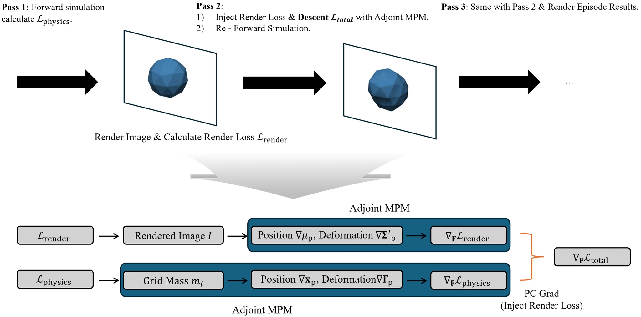
6.
Gradient fusion and control update
•
Rendering gradients flow back through the renderer, covariance mapping, F‑interpolation, and subdivision to the anchor deformation controls.
•
In parallel, physics gradients from the grid‑mass objective are obtained via adjoint MPM.
•
We fuse the two gradient sources with PCGrad and magnitude normalization, then update Control Deformation Gradient using Adam, closing the loop for render‑informed physics optimization.
7.
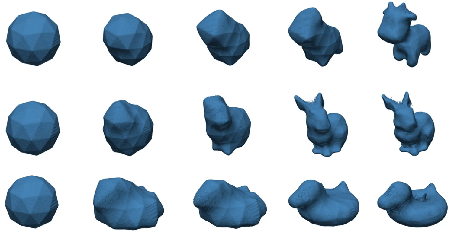
Results
•
Sphere to Bunny
•
Sphere to Spot
